3.8 | Preparing the sales forecast fact table (factForecast)
In the previous chapter we prepared the fact table factSales which contains the actual sales transactions that happened over time. In many real-world use-cases plan data is integrated in the BI solution in order to allow comparisons and better judge performance.
For our example use-case we have a table with forecasted sales data which we want to integrate into the data model. Let's prepare the table.
1. Navigate to the table factForecast
2. Delete the automatically generated step Changed Type
3. Promote the top row to become the table headers
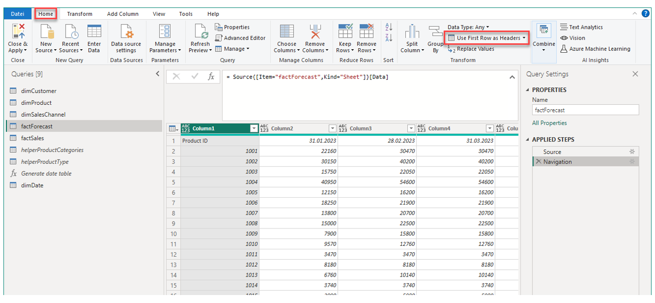
4. Delete the automatically generated step Changed Type
When promoting a row to become table headers, Power Query always attempts to guess the right data type for each column and creates a transformation step accordingly. We do that later and therefore please delete this step.
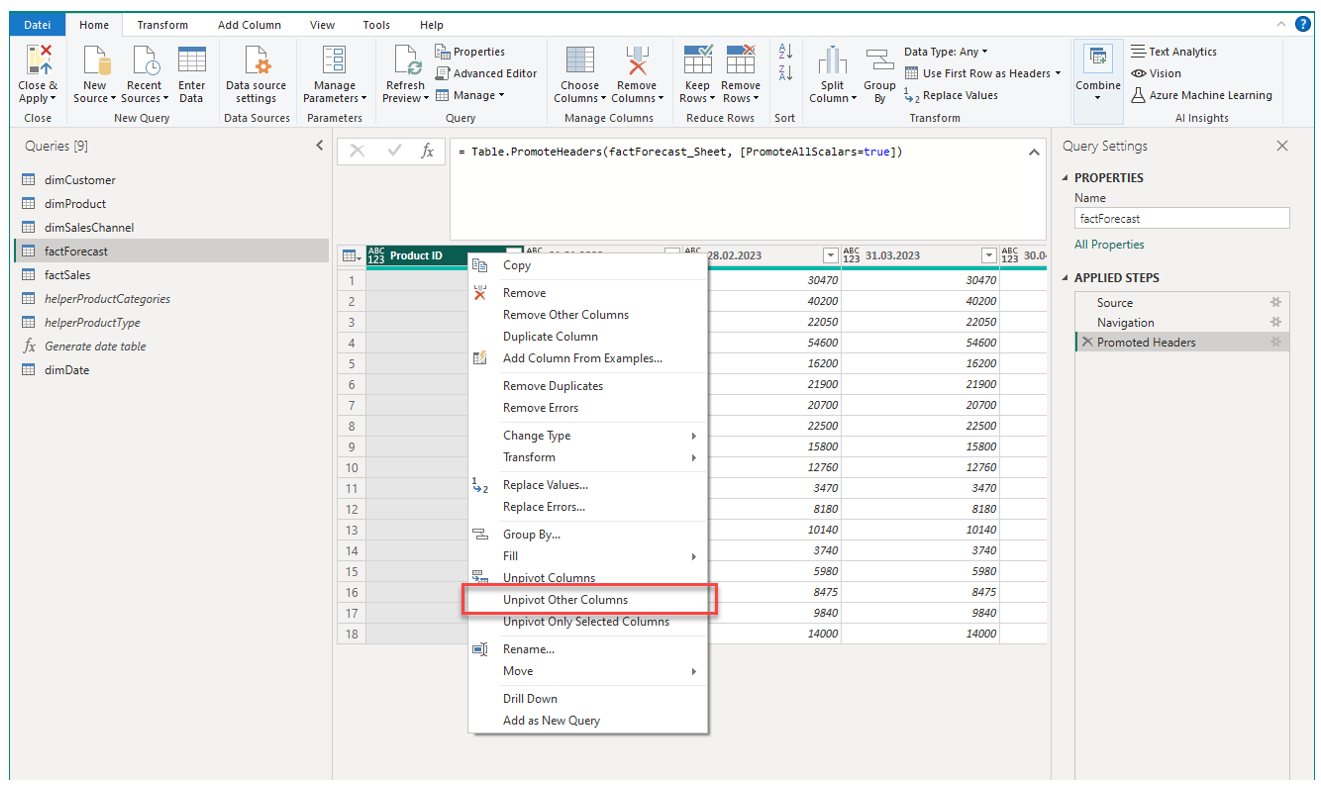
5. Unpivot the columns containing forecast values
Now when we inspect the table, we can see that apart from Product ID, each column has a particular month in date format as its column header. This is a typical format with which planning data is generated. It is however not a useful structure when working with a BI tool.
To restructure the table into a more useful format, we simply unpivot all columns except Product ID. To do that, do a right-click on the column header of Product ID and select Unpivot Other Columns:
The table then should look like this:
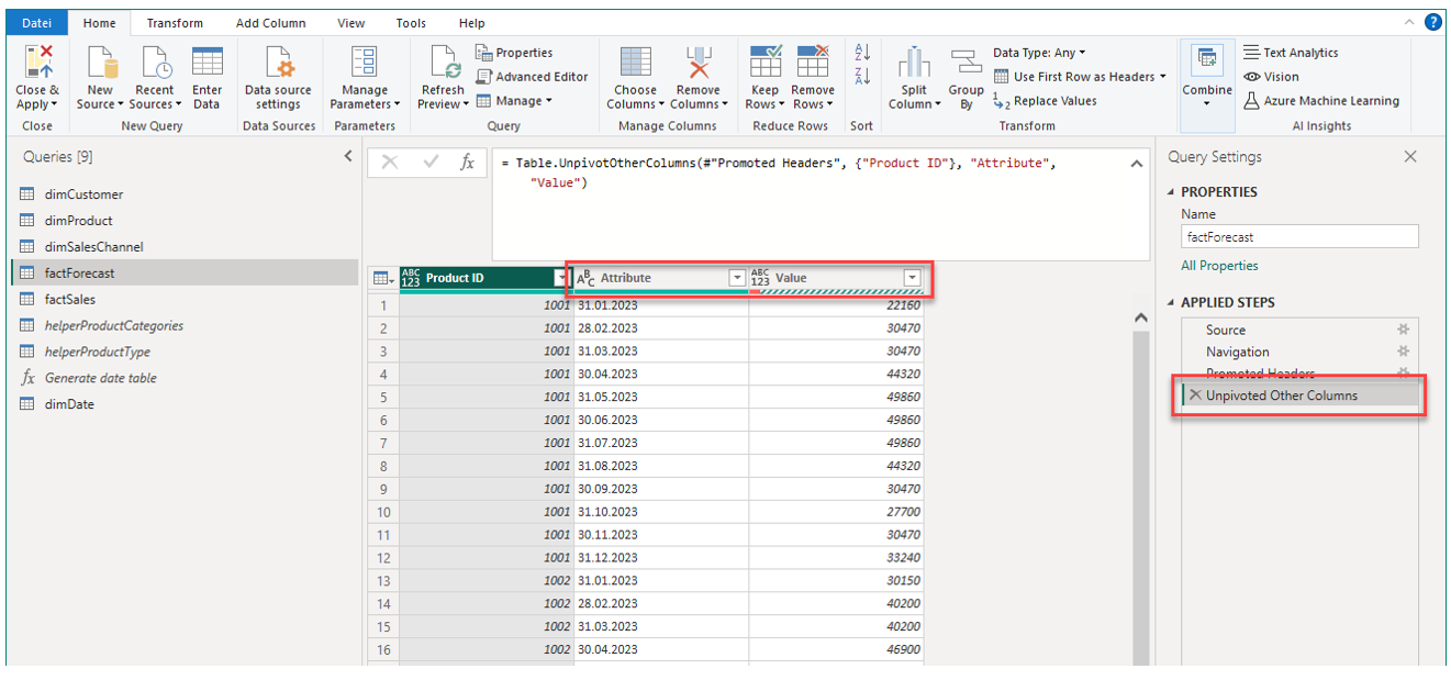
As you can see, the previous table headers are now stored in a new column Attribute and the respective forecast values are in the column Value. Let's rename these table headers in the next step.
6. Rename the newly created columns
Rename Attribute to Date and Value to Sales in USD respectively. Remember, either do a double-click on the header name to rename or a right-click and select Rename.
7. Set the data type for all columns
Convert the column Date to data type date, Sales in USD to Decimal number and Product ID to data type text.
8. Clean the table from errors
Upon inspecting the table preview, Power Query tells us that there are errors in the column Sales in USD. There is an indication just below the table header that tells us the quality and completness of a column (see further below for more details). If you scroll down a bit in the table, you should see the errors.
When clicking into the cell of one of the errors (NOT on the text Error), Power Query shows the error message in yellow:
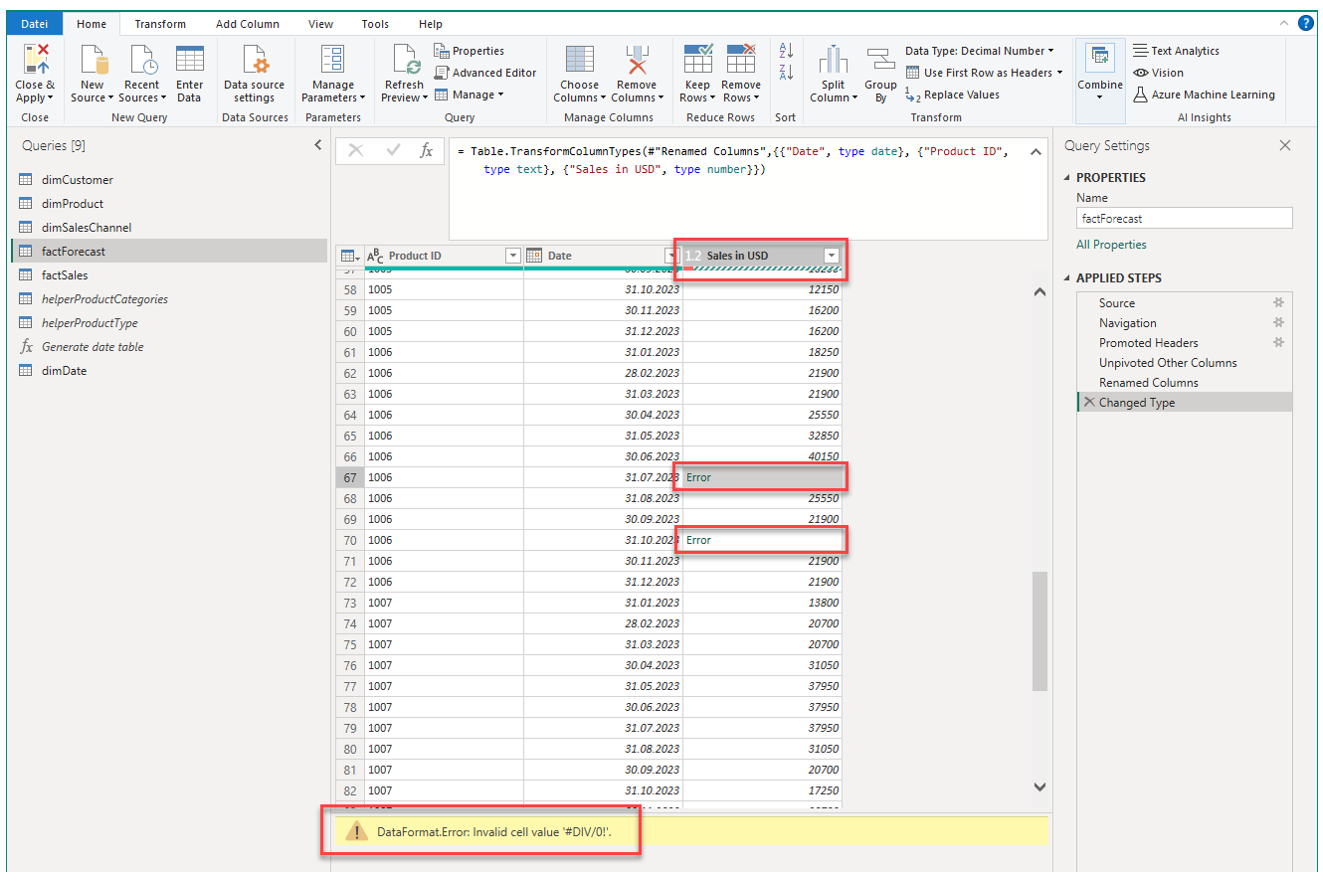
It seems that there are formula errors in the underlying Excel table (#DIV/0). Note, this is a very common occurence when working with Excel files as data sources.
Usually we would not go back to the provider of the forecast data and let the errors be fixed and replaced with the proper values. For our demo use-case we now simply replace the errors with zeros in order to be able to move on and load the table to the data model. Like this, you also learn a new transformation step. However, please feel free to enter some figures in the erroneous cells in the Excel file (make sure to hit Refresh Preview after saving the changes to the Excel file in order to see the changes in Power Query).
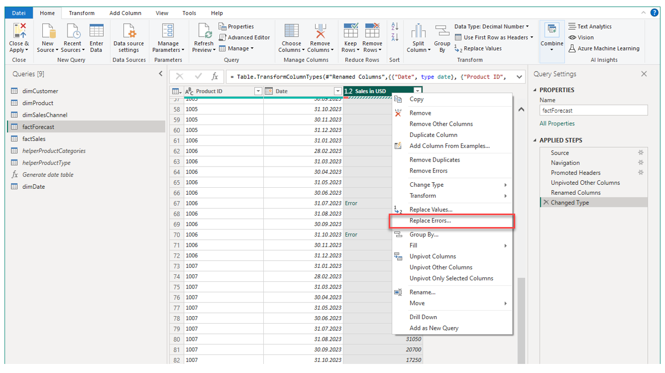
Simply do a right-click on the respective column header and select Replace Errors:
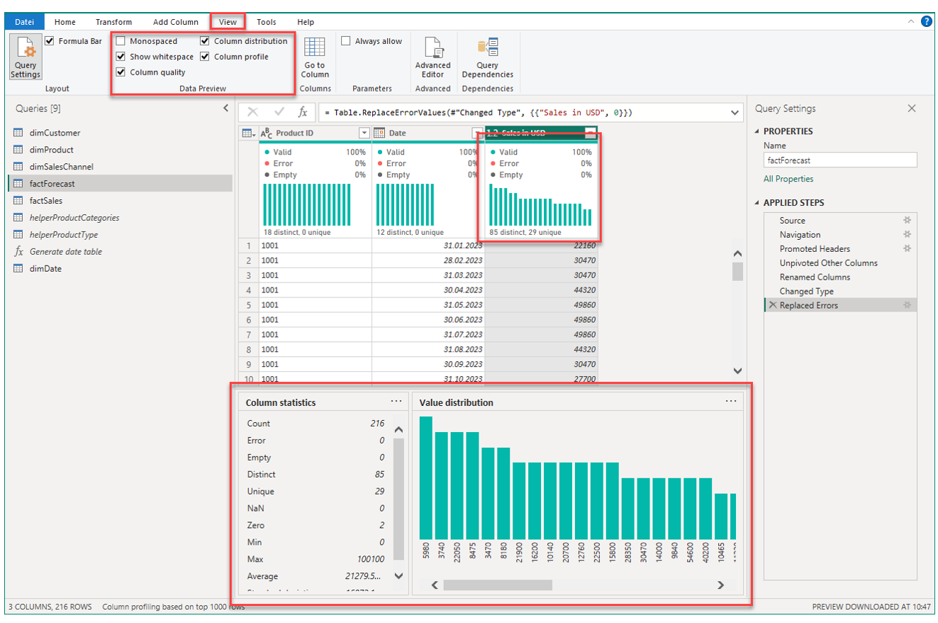
In the appearing window, enter a zero and confirm with OK:

The errors should be gone and there should not be any indication red indication just below the column header.
Under View → Data Preview there are different features to analyze the quality and profile of the table columns.
We are now down with preparing all tables. In the following chapter, we will tidy up Power Query and load the data to the data model.